
The NLSY97 sampling weights, which are constructed in each survey year, provide the researcher with an estimate of how many individuals in the United States are represented by each NLSY97 respondent. Individual case weights are assigned to produce group population estimates when used in tabulations.
This sampling weights section includes the following information:
- Introduction to weighting
- Types of weights
- Practical usage of weights
- Methodology for calculating weights
- Summary of NLSY97 weights by round
- Design effects
Important information: Custom Weights
Custom Weights for the NLSY97 are provided online for users needing longitudinal weights for multiple survey years or for a specific set of respondent ids.
Introduction to weighting
Weighting is a challenging subject. Researchers must first decide if they should or should not weight the sample. If researchers decide to weight, they must then determine which weight variable to use. This can be a difficult decision because there are more than 30 different pre-created weight variables available in the NLSY97 dataset.
What does weighting do? Weights are in place to make sure the sample is representative of the population of interest and that other objectives are met. Weights are particularly important when over-sampling occurs. All NLS data sets use over-sampling. Over-sampling is the selection of a large number of additional respondents that match certain criteria. This over-sampling was done to allow researchers to measure more precisely the changes in key populations like blacks and Hispanics. Over-sampling impacts population descriptors, such as means and medians, because the NLSY97 has more respondents who are black or Hispanic than what really exists in the U.S. If the data are not adjusted, the greater number of black and Hispanic respondents skews population averages toward black and Hispanic averages. Adjusting the data by weighting reduces the impact of each black and Hispanic respondent and removes that bias. If a user attempts to summarize characteristics of the population but ignores weights, results are biased.
Weights for the NLSY97 range from a high of around 1.7 million to a low of 86,000. What do these numbers mean? All NLSY97 weights contain two implied decimal places. To interpret the weight, divide by 100. For example, a respondent with a weight of 1.7 million represents 17,000 people, while a respondent with weight of 86,000 represents 860 people. If a NLSY97 respondent has a weight of 0, he or she did not participate in that survey round.
Important information: Descriptive statistics
If you are creating descriptive statistics such as means, medians, and standard deviations, it is suggested that you weight your results. If you are running a more complex analysis such as doing a regression, we suggest that you do not weight. For more details on when to use weights, see Practical Usage of Weights.
Types of weights
Weights are found under the "Sample Design & Screening" Area of Interest in Investigator. Weights also can be found by searching for the word "Weight" in the Word in Title search option. There are three sampling weight variables available in each round:
SAMPLING_WEIGHT_CC. Provides a weight for everyone who participated in that particular round of surveying, using a special method of combining the cross-sectional and over-sample cases. This method makes the weight of an oversampled person invariant to which sample the person was drawn from. This reduces the variation in weights and hence improves the statistical efficiency of weighted estimators.
SAMPLING_PANEL_WEIGHT. This weights only people who are in every round from 1 to N. Those not in every round get a 0 weight. It is used when data are needed on individuals who participated in all rounds.
MORTADJ_SAMPWEIGHT. Provides a weight allowing for population estimates for the portion of the base year population that is still alive as of the given round of surveying. It has been calculated by adjusting the SAMPLING_WEIGHT_CC methodology to account for mortality within the panel. This is done by modifying the poststratification benchmarks to remove the portion of the base year population estimated to be deceased by the particular round of surveying.
Rounds 1 and 2 also include two additional sampling weight variables, SAMPLING_WEIGHT and CS_SAMPLING_WEIGHT. Starting in round 3, NLS survey staff created a new, more statistically efficient method of calculating survey weights called the "Cumulating Cases" strategy. Because the new method provided better information, weights were recalculated starting with round 1. However, since research had already been published using the original sampling weight variables, the original variables were left in the database to enable older work to be replicated.
For more details about how the weights were calculated, see Methodology for calculating weights.
Important information: Weight check
Need a quick check to see the impact of weights for a complex statistical situation? Use R12361.01, which is the Round 1 Sampling Weight Cumulative Cases Method. This variable provides a weight for every NLSY97 respondent and adjusts for the over-sampling of blacks and Hispanics. It does not adjust for round-by-round non-response.
Practical usage of weights
Researchers should weight the observations using the weights provided if tabulating sample characteristics in order to describe the population represented (i.e., computing sample means, totals, or proportions). The use of weights may not be appropriate without other adjustments for the following applications:
Samples generated by dropping observations with item nonresponses
Often users confine their analysis to subsamples of respondents who provided valid answers to certain questions. In this case, a weighted mean will not represent the entire population, but rather those persons in the population who would have given a valid response to the specified questions. Item nonresponse due to refusals, don't knows, or invalid skips is usually quite small, so the degree to which the weights are incorrect is probably quite small. In the event that item nonresponse constitutes a small proportion of the variables under analysis, population estimates (i.e., weighted sample means, medians, and proportions) are reasonably accurate. However, population estimates based on data items that have relatively high nonresponse rates--such as family income--may not necessarily be representative of the underlying population of the cohort under analysis.
Data from multiple waves
Because the weights are specific to a single wave of the study, and because respondents occasionally miss an interview but are contacted in a subsequent wave, a problem similar to item nonresponse arises when the data are used longitudinally. In addition, the weights for a respondent in different years occasionally may be quite dissimilar, leaving the user uncertain as to which weight is appropriate. In principle, if a user wished to apply weights to multiple wave data, weights would have to be recomputed based upon the persons for whom complete data are available. In practice, if the sample is limited to respondents interviewed in a terminal or end point year, the weight for that year can be used.
Users may also create longitudinal weights for multiple survey years by using the NLSY97 Custom Weighting program.
Regression analysis
A common question is whether one should use the provided weights to perform weighted least squares when doing regression analysis. Such a course of action may lead to incorrect estimates. If particular groups follow significantly different regression specifications, the preferred method of analysis is to estimate a separate regression for each group or to use indicator variables to specify group membership; regression on a random sample of the population would be misspecified. Users uncertain about the appropriate method should consult an econometrician, statistician, or other person knowledgeable about the data before specifying the regression model.
Analysis by race
For research that includes analysis by race, using the regular sampling weights rather than the cross-sectional weights will produce results with higher precision for black and Hispanic or Latino youths. For research that focuses only on non-black, non-Hispanic youths or that does not include any analysis by race/ethnicity, using the cross-sectional weights will save processing time.
Methodology for calculating weights
The assignment of individual respondent weights involved a number of different adjustments. Complete details are found in the NLSY97 Technical Sampling Report, which has step-by-step descriptions of the entire adjustment process. Some of the major adjustments are:
- Adjustment One. Computation of a base weight, reflecting the case's selection probability for the screening sample. This step also corrects for missed housing units and caps the base weights in the supplemental sample to prevent extremely high weights;
- Adjustment Two. Adjustment for nonresponse to the screener;
- Adjustment Three. Development of a combination weight to allow the black and Hispanic cases from the cross-sectional sample to be merged with those from the supplemental sample (non-Hispanic, non-blacks in the supplemental sample were not eligible for the NLSY97 sample);
- Adjustment Four. Adjustment of the weights for nonresponse to NLSY97 interviews;
- Adjustment Five. Poststratification of the nonresponse-adjusted weights to match national totals.
Calculation of weights under new 'Cumulating Cases' strategy
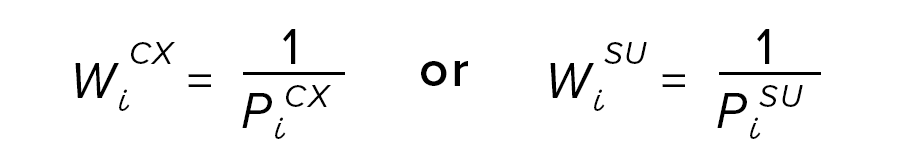
Starting in round 4, a new 'Cumulating Cases' strategy has been used to calculate weights. Instead of calculating separate CX and SU (cross-sectional and supplemental) base weights and then later combining the separate sample weights, a Horvitz-Thompson approach to weighting is used.
In the Horvitz-Thompson approach, the weights are determined across samples depending only on the overall selection probability (into either sample) of the individual element, giving a single, unified set of weights for the cumulated cases. This approach is straightforward. Only Adjustments 1 and 3 above are modified. The probability for a case to be in either sample is simply the sum of the probabilities to be in each sample because the samples are independently drawn. Thus, the base weight for a case is the inverse of the sum of sample selection probabilities for a case:

where
PiCX = sel. prob. for case i in CX sample, and
PiSU = sel. prob. for case i in SU sample.
Under the old strategy, the separate CX and SU step 1 weights were the reciprocal of the selection probabilities for just that sample:
The only other change is that Adjustment 3 is now unnecessary.
Calculation of the Mortality Adjusted Weights
Mortality Adjusted Weights are calculated for Rounds 2 and later using the Cumulating Cases strategy as a starting point, but then modifying the poststratification step so that the benchmarks account for mortality. Mortality-adjusted benchmarks for a particular round N>1 are computed in a way that uses the Round 1 CC weights, in combination with information on whether panelists are alive as of Round N, to estimate population sizes (by poststrata) for the portion of the base year population that is still living as of round N. Specifically, the mortality-adjusted benchmarks for a particular round N>1 are computed by summing the Round 1 SAMPLING_WEIGHT_CC weight within poststratification cell among panelists not known to be deceased by round N. These mortality-adjusted benchmarks are then used to poststratify the weights of respondents in that round.
Summary of NLSY97 weights by round
Table 1 summarizes the weights for each of the NLSY97 rounds. The sum of the weights for all of these weights is equal, but when there are fewer positive weights to share this sum, the weights tend to increase. The positive weights for Round 1 respondents who are nonrespondents for any of the other rounds are spread around the round's (or panel's) respondents.
Scroll right to view additional table columns or click the link at the bottom of the table to open in a new window.
| Round | Round Year | Descriptive Statistics | ||||||||||
|---|---|---|---|---|---|---|---|---|---|---|---|---|
| N (>0) | Sum | Mean | Standard Deviation | Min. (>0) | 5th Percentile | 25th Percentile | Median | 75th Percentile | 95th Percentile | Max. | ||
| 1 | 1997 | 8,984 | 19,378,453 | 2,157.00 | 931.01 | 760.71 | 887.2 | 1,072.03 | 2,596.59 | 2,909.73 | 3,268.16 | 15,761.82 |
| 2 | 1998 | 8,386 | 19,378,454 | 2,310.81 | 1,011.70 | 846.23 | 938.12 | 1,135.96 | 2,777.05 | 3,111.65 | 3,556.58 | 16,718.19 |
| 3 | 1999 | 8,209 | 19,378,453 | 2,360.64 | 1,021.15 | 858.76 | 969 | 1,168.73 | 2,806.46 | 3,154.13 | 3,649.77 | 16,646.80 |
| 4 | 2000 | 8,081 | 19,378,453 | 2,398.03 | 1,052.08 | 889.08 | 983.16 | 1,185.60 | 2,869.30 | 3,203.60 | 3,786.59 | 16,950.37 |
| 5 | 2001 | 7,883 | 19,378,453 | 2,458.26 | 1,066.22 | 866.55 | 997.49 | 1,222.83 | 2,955.45 | 3,271.03 | 3,831.66 | 17,277.02 |
| 6 | 2002 | 7,898 | 19,378,453 | 2,453.59 | 1,092.47 | 864.75 | 992.86 | 1,204.79 | 2,955.01 | 3,293.50 | 3,904.73 | 17,167.26 |
| 7 | 2003 | 7,756 | 19,378,454 | 2,498.51 | 1,118.88 | 900.6 | 1,006.25 | 1,230.15 | 3,009.67 | 3,356.67 | 3,997.80 | 17,852.01 |
| 8 | 2004 | 7,503 | 19,378,453 | 2,582.76 | 1,162.17 | 868.23 | 1,016.25 | 1,273.38 | 3,144.57 | 3,458.88 | 4,158.40 | 18,026.17 |
| 9 | 2005 | 7,338 | 19,378,453 | 2,640.84 | 1,200.80 | 916.66 | 1,037.19 | 1,263.82 | 3,215.89 | 3,579.02 | 4,183.79 | 18,594.09 |
| 10 | 2006 | 7,559 | 19,378,454 | 2,563.63 | 1,157.31 | 918.64 | 1,022.26 | 1,230.84 | 3,124.67 | 3,469.62 | 4,044.36 | 18,521.05 |
| 11 | 2007 | 7,418 | 19,378,453 | 2,612.36 | 1,180.74 | 897.41 | 1,046.29 | 1,267.50 | 3,178.10 | 3,541.70 | 4,127.30 | 18,857.91 |
| 12 | 2008 | 7,490 | 19,378,455 | 2,587.20 | 1,178.50 | 894 | 1,024.90 | 1,254.40 | 3,146.90 | 3,534.60 | 4,054.50 | 19,165.40 |
| 13 | 2009 | 7,559 | 19,378,453 | 2,563.63 | 1,175.61 | 866.01 | 997.75 | 1,235.94 | 3,144.54 | 3,516.00 | 4,012.05 | 18,911.82 |
| 14 | 2010 | 7,479 | 19,378,452 | 2,591.05 | 1,201.68 | 876.7 | 1,011.30 | 1,231.02 | 3,155.05 | 3,563.37 | 4,118.80 | 19,222.75 |
| 15 | 2011 | 7,423 | 19,378,452 | 2,610.60 | 1,225.20 | 882.87 | 1,020.56 | 1,242.24 | 3,167.25 | 3,597.63 | 4,232.26 | 19,377.82 |
| 16 | 2013 | 7,141 | 19,378,452 | 2,713.69 | 1,271.64 | 891.34 | 1,050.96 | 1,278.73 | 3,327.70 | 3,754.63 | 4,310.88 | 20,094.05 |
| 17 | 2015 | 7,103 | 19,378,454 | 2,728.21 | 1,282.70 | 890.61 | 1,064.28 | 1,282.44 | 3,390.06 | 3,755.54 | 4,380.94 | 19,803.54 |
| 18 | 2017 | 6,734 | 19,378,453 | 2,877.70 | 1,318.34 | 926.76 | 1,093.74 | 1,378.47 | 3,525.73 | 3,903.84 | 4,586.40 | 20,072.81 |
| 19 | 2019 | 6,947 | 19,378,453 | 2,789.47 | 1,275.79 | 918.04 | 1,076.51 | 1,346.11 | 3,397.94 | 3,786.88 | 4,441.97 | 20,043.66 |
| 20 | 2021 | 6,713 | 19,378,452 | 2,886.71 | 1,351.23 | 937.37 | 1,090.59 | 1,359.18 | 3,527.77 | 3,978.75 | 4,626.92 | 21,090.85 |
| 21 | 2023 | 6,569 | 19,378,452 | 2,949.99 | 1,381.53 | 939.89 | 1,108.39 | 1,380.50 | 3,625.96 | 4,064.90 | 4,734.89 | 21,662.43 |
Design effects
Calculating design-corrected standard errors for NLSY97: Overview
The National Longitudinal Survey of Youth, 1997 (NLSY97) is a combination of two area-probability samples. The Cross-Sectional (CX) sample is an equal-probability multi-stage cluster sample of housing units for the entire United States (every housing unit in the United States in 1997 had an equal probability of being in the CX sample). The Supplemental (SU) Sample is a multi-stage cluster sample of housing units that oversamples Hispanic and non-Hispanic Black youths; it is designed so that every eligible Hispanic and non-Hispanic Black youth in the United States in a housing unit in 1997 had an equal probability of being in the SU sample.
Since these samples are cluster samples, standard errors are larger for the NLSY97 than simple random sample calculations (calculated without correction for the design) would indicate. To correctly calculate standard errors, design variables must be used in statistical software. Without these design variables, statistical software will assume a simple random sample and underestimate standard errors. For a handful of variables selected below in Table 1, we see multiplier effects on standard errors (labeled DEFT) ranging from 1.30 to 1.62.
In order to facilitate the calculation of design effects, we provide two design variables for every Round 1 NLSY97 interview: VSTRAT and VPSU. VSTRAT is the Variance STRATum while VPSU is the Variance Primary Sampling Unit. The combination of VSTRAT and VPSU reflect the first-stage and second-stage units selected as part of the NORC National Sampling Frame. There are two second-stage units (VPSU) for each first-stage unit (VSTRAT).
First stage units in the NLSY97 are called Primary Sampling Units (PSUs), each of which is composed of one or more counties. The largest urban areas are selected with certainty to guarantee their representation in NSLY97. Second-stage stage units in the NLSY97 are called segments, each of which is one or more Census-defined blocks. The first-stage and second-stage units are selected with probabilities proportional to size (housing units for the CX sample; minority youths for the SU sample), and the sample housing units (third-stage units) are then selected to be an equal-probability sample.
To create the variables VSTRAT and VPSU, we recode the PSUs and segments, depending on whether the PSU was selected with certainty. Certainty PSUs are considered strata, so all the segments in one certainty PSU are in one VSTRAT value, with segments divided so that half are assigned to VPSU = 1 while the other half are assigned to VPSU = 2. Some certainty PSUs are large enough to be divided into multiple VSTRAT values with up to twenty segments in one VSTRAT value (ten in each VPSU). Non-certainty PSUs are paired into one VSTRAT value with one PSU assigned to VPSU = 1 while the other PSU is assigned to VPSU = 2. It is rare, but possible, for PSUs to be combined in one VPSU. This strategy was designed by Kirk Wolter.
Here is sample Stata code to analyze the variable ANALYSISVAR within an NLSY97DATAFILE with the appropriate weight variable for the analysis, WTVAR:
use NLSY97DATAFILE.dta,clear
svyset [pweight=WTVAR], strata(vstrat) psu(vpsu) singleunit(scaled)
svy: mean ANALYSISVAR //mean for continuous variables
svy: proportion ANALYSISVAR //proportion for categorical variables
estat effects //design effects--this generates the DEFF and DEFT
svy, subpop (if SUBGROUP==1): mean ANALYSISVAR // mean within a subpopulation
svy: tabulate ANALYSISVAR //one way table
The results generated by running this code on select NLSY97 variables are shown in Table 4. They report design-corrected standard errors as well as standard errors assuming simple random sampling as would be estimated in the absence of these design variables.
|
Variable |
Mean/ |
Sample Size |
Estimate |
Design-corrected |
SRS |
DEFF |
DEFT |
|---|---|---|---|---|---|---|---|
|
Gross family income 2009 from 2010 interview [T5206900] |
Mean | 6527 | 64858.5 | 923.831 | 773.64 | 1.728 | 1.314 |
|
ASVAB score for Math (percentile) [R9829600] |
Mean | 7093 | 50.410 | 0.638 | 0.367 | 3.447 | 1.857 |
|
ASVAB score for Math (percentile) for females [R9829600, R0536300] |
Mean | 8102 | 51.508 | 0.705 | 0.509 | 2.222 | 1.491 |
|
Weeks worked in 2008 [Z9061800] |
Mean | 8011 | 40.021 | 0.270 | 0.224 | 1.700 | 1.304 |
|
Ever received a bachelor's degree or higher as of 2011 interview [T6657200] |
Proportion | 7398 | 0.300 | 0.009 | 0.006 | 2.614 | 1.617 |
|
Never received a high school diploma as of 2011 interview [T6657200] |
Proportion | 7398 | 0.199 | 0.007 | 0.005 | 2.368 | 1.539 |
|
Lived with 2 parents (at least 1 bioparent) in Round 1 [R1205300] |
Proportion | 8953 | 0.675 | 0.007 | 0.005 | 2.216 | 1.489 |
|
Note: Tabulations use the Round 1 Cumulating Cases Sampling Weight [R1236101]. |
|||||||
One thing to note is that the sample size for math ASVAB scores for females is greater than the sample size for math ASVAB scores for all respondents. Though the estimate uses only the 3503 observations of females with non-missing data for ASVAB scores, the variance calculation uses information from all observations in the data whether or not they have valid values for the specific variables. (See How can I analyze a subpopulation of my survey data in STATA? for more information.)
In SAS, one would use PROC SURVEYFREQ to calculate the design-corrected standard errors. SPSS is menu-driven, so no code is given here, but you can create design-corrected standard errors within SPSS using the Complex Samples add-on.
Potential problems with sparse data
If you are calculating design-corrected standard errors using a subsample of the NLSY97 data set and/or using a variable that has a large number of observations with missing values, you may receive a message such as this:
STATA error handling: "missing standard error because of stratum with single sampling unit"
VSTRAT and VPSU were created so that there was a minimum of 7 NLSY97 respondents within a VSTRAT/VPSU cell. However, if all respondents within a cell are missing on a variable, it will be impossible to calculate the standard error. If the dataset is subset (to males or females, for example), this error becomes more likely to happen.
The best workaround is to merge two VSTRATA together to eliminate this problem (the VSTRATA are ordered so that similar VSTRATA are numerically consecutive). To diagnose the problem, run a frequency of the data by VSTRAT/VPSU and look for VSTRAT values with only one VPSU with respondents. Here is an example:
|
VSTRAT |
VPSU |
# of cases |
|---|---|---|
| … | … | … |
| x-1 | 1 | 3 |
| x-1 | 2 | 5 |
| X | 1 | 4 |
| x+1 | 1 | 6 |
| x+1 | 2 | 4 |
| … | … | … |
The error occurs because VSTRAT = x has four cases with VPSU=1 but none with VPSU=2. This prevents Stata from calculating the variance for this strata (it has nothing to compare VPSU=1 with). The cases were sorted by VSTRAT and VPSU so that the most similar VSTRATA are numbered consecutively and the most similar cases are always within the two VPSU values of one VSTRAT value. The easiest solution is therefore to make room for VSTRAT x within VSTRAT x-1 by combining the two VPSUs within VSTRAT x-1. Then, the VSTRAT x cases are moved to the other VSPU value within VSTRAT x-1. Note that VSTRAT x-1 is chosen instead of VSTRAT x+1 in this example because VSTRAT x-1 has fewer total cases (8) than VSTRAT x+1 (10). In some, but not all cases, the VPSU 1 cases in VSTRAT x are "more similar" to the VSTRAT x-1 cases than the VSTRAT x+1 cases. Here are the two programming steps:
- If VSTRAT = x-1 and VPSU = 2 then VPSU=1
- If VSTRAT = x then VSTRAT=x-1 and VPSU=2.
Here is the revised frequency:
|
VSTRAT |
VPSU |
# of cases |
|---|---|---|
| … | … | … |
| x-1 | 1 | 8 |
| x-1 | 2 | 4 |
| x+1 | 1 | 6 |
| x+1 | 2 | 4 |
| … | … | … |
This eliminates the "stratum with a single sampling unit." In severe cases of data subsets, this step may be required more than once, although this may also indicate that the "clustering" has been removed (by using less than 10 percent of the total sample, for example).